Optimization of an X-Gate for a Transmon Qubit

# NBVAL_IGNORE_OUTPUT
%load_ext watermark
import qutip
import numpy as np
import scipy
import matplotlib
import matplotlib.pylab as plt
import krotov
%watermark -v --iversions

qutip       4.3.1
numpy       1.15.4
scipy       1.1.0
matplotlib  3.0.2
matplotlib.pylab  1.15.4
krotov      0.0.1
CPython 3.6.7
IPython 7.2.0

\(\newcommand{tr}[0]{\operatorname{tr}} \newcommand{diag}[0]{\operatorname{diag}} \newcommand{abs}[0]{\operatorname{abs}} \newcommand{pop}[0]{\operatorname{pop}} \newcommand{aux}[0]{\text{aux}} \newcommand{opt}[0]{\text{opt}} \newcommand{tgt}[0]{\text{tgt}} \newcommand{init}[0]{\text{init}} \newcommand{lab}[0]{\text{lab}} \newcommand{rwa}[0]{\text{rwa}} \newcommand{bra}[1]{\langle#1\vert} \newcommand{ket}[1]{\vert#1\rangle} \newcommand{Bra}[1]{\left\langle#1\right\vert} \newcommand{Ket}[1]{\left\vert#1\right\rangle} \newcommand{Braket}[2]{\left\langle #1\vphantom{#2} \mid #2\vphantom{#1}\right\rangle} \newcommand{op}[1]{\hat{#1}} \newcommand{Op}[1]{\hat{#1}} \newcommand{dd}[0]{\,\text{d}} \newcommand{Liouville}[0]{\mathcal{L}} \newcommand{DynMap}[0]{\mathcal{E}} \newcommand{identity}[0]{\mathbf{1}} \newcommand{Norm}[1]{\lVert#1\rVert} \newcommand{Abs}[1]{\left\vert#1\right\vert} \newcommand{avg}[1]{\langle#1\rangle} \newcommand{Avg}[1]{\left\langle#1\right\rangle} \newcommand{AbsSq}[1]{\left\vert#1\right\vert^2} \newcommand{Re}[0]{\operatorname{Re}} \newcommand{Im}[0]{\operatorname{Im}}\)

Define the Hamiltonian

The effective Hamiltonian of a single transmon depends on the capacitive energy \(E_C=e^2/2C\) and the Josephson energy \(E_J\), an energy due to the Josephson junction working as a nonlinear inductor periodic with the flux \(\Phi\). In the so-called transmon limit the ratio between these two energies lie around \(E_J / E_C \approx 45\). The time-independent Hamiltonian can be described then as

\begin{equation*} \op{H}_{0} = 4 E_C (\hat{n}-n_g)^2 - E_J \cos(\hat{\Phi}) \end{equation*}

where \(\hat{n}\) is the number operator, which count how many Cooper pairs cross the junction, and \(n_g\) being the effective offset charge measured in Cooper pair charge units. The aforementioned equation can be written in a truncated charge basis defined by the number operator \(\op{n} \ket{n} = n \ket{n}\) such that

\begin{equation*} \op{H}_{0} = 4 E_C \sum_{j=-N} ^N (j-n_g)^2 |j \rangle \langle j| - \frac{E_J}{2} \sum_{j=-N} ^{N-1} ( |j+1\rangle\langle j| + |j\rangle\langle j+1|). \end{equation*}

If we apply a potential \(V(t)\) to the qubit the complete Hamiltonian is changed to

\begin{equation*} \op{H} = \op{H}_{0} + V(t) \cdot \op{H}_{1} \end{equation*}

The interaction Hamiltonian \(\op{H}_1\) is then equivalent to the charge operator \(\op{q}\), which in the truncated charge basis can be written as

\begin{equation*} \op{H}_1 = \op{q} = \sum_{j=-N} ^N -2n \ket{n} \bra{n}. \end{equation*}

Note that the -2 coefficient is just indicating that the charge carriers here are Cooper pairs, each with a charge of \(-2e\).

We define the logic states \(\ket{0_l}\) and \(\ket{1_l}\) (not to be confused with the charge states \(\ket{n=0}\) and \(\ket{n=1}\)) as the eigenstates of the free Hamiltonian \(\op{H}_0\) with the lowest energy. The problem to solve is find a potential \(V_{opt}(t)\) such that after a given final time \(T\) can

def transmon_ham_and_states(Ec=0.386, EjEc=45, nstates=8, ng=0.0, T=10.0, steps=1000):
    """Transmon Hamiltonian"""
    # Ec       :  capacitive energy
    # EjEc     :  ratio Ej / Ec
    # nstates  :  defines the maximum and minimum states for the basis. The truncated basis
    #             will have a total of 2*nstates + 1 states

    Ej = EjEc * Ec
    n = np.arange(-nstates, nstates+1)
    up = np.diag(np.ones(2*nstates),k=-1)
    do = up.T
    H0 = qutip.Qobj(np.diag(4*Ec*(n - ng)**2) - Ej*(up+do)/2.0)
    H1 = qutip.Qobj(-2*np.diag(n))

    eigenvals, eigenvecs = scipy.linalg.eig(H0.full())
    ndx = np.argsort(eigenvals.real)
    E = eigenvals[ndx].real
    V = eigenvecs[:,ndx]
    w01 = E[1]-E[0] # Transition energy between states

    psi0 = qutip.Qobj(V[:, 0])
    psi1 = qutip.Qobj(V[:, 1])

    profile = lambda t: np.exp(-40.0*(t/T - 0.5)**2)
    eps0 = lambda t, args: 0.5 * profile(t) * np.cos(8*np.pi*w01*t)
    return ([H0, [H1, eps0]], psi0, psi1)

H, psi0, psi1 = transmon_ham_and_states()

We introduce the projectors \(P_i = \ket{\psi _i}\bra{\psi _i}\) for the logic states \(\ket{\psi _i} \in \{\ket{0_l}, \ket{1_l}\}\)

proj0 = psi0 * psi0.dag()
proj1 = psi1 * psi1.dag()

Optimization target

We choose our X-gate to be defined during a time interval starting at \(t_{0} = 0\) and ending at \(T = 10\), with a total of \(nt = 1000\) time steps.

tlist = np.linspace(0, 10, 1000)

We make use of the \(\sigma _{x}\) operator included in QuTiP to define our objective:

objectives = krotov.gate_objectives(
    basis_states=[psi0, psi1], gate=qutip.operators.sigmax(), H=H)

We define the desired shape of the pulse and the update factor \(\lambda _a\)

def S(t):
    """Shape function for the pulse update"""
    dt = tlist[1] - tlist[0]
    steps = len(tlist)
    return np.exp(-40.0*(t/((steps-1)*dt)-0.5)**2)

pulse_options = {
    H[1][1]: krotov.PulseOptions(lambda_a=1, shape=S)
}

It may be useful to check the fidelity after each iteration. To achieve this, we define a simple function that will be used by the main routine

def print_fidelity(**args):
    F_re = np.average(np.array(args['tau_vals']).real)
    print("Iteration %d: \tF = %f" % (args['iteration'], F_re))
    return F_re

Simulate dynamics of the guess pulse

def plot_pulse(pulse, tlist):
    fig, ax = plt.subplots()
    if callable(pulse):
        pulse = np.array([pulse(t, None) for t in tlist])
    ax.plot(tlist, pulse)
    ax.set_xlabel('time')
    ax.set_ylabel('pulse amplitude')
    plt.show(fig)

plot_pulse(H[1][1], tlist)

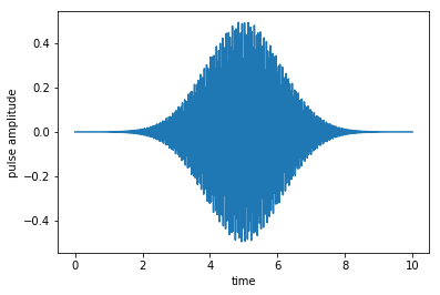
Once we are sure to have obtained the desired guess pulse, the dynamics for the initial guess can be found easily

guess_dynamics = [objectives[x].mesolve(tlist, e_ops=[proj0, proj1]) for x in [0,1]]
# using initial state psi0 = objectives[0].initial_state

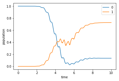
def plot_population(result):
    fig, ax = plt.subplots()
    ax.plot(result.times, result.expect[0], label='0')
    ax.plot(result.times, result.expect[1], label='1')
    ax.legend()
    ax.set_xlabel('time')
    ax.set_ylabel('population')
    plt.show(fig)

plot_population(guess_dynamics[0])
plot_population(guess_dynamics[1])

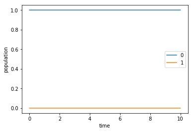
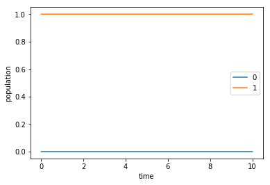
It is obvioius that our initial guess is not even near the pulse that we are trying to achieve. However we will still use it and try to see what results that we can obtain.

Optimize

We now use all the information that we have gathered to initialize the optimization routine. That is:

• The objectives: creating an X-gate in the given basis.
• The pulse_options: initial pulses and their shapes restrictions.
• The tlist: time grid used for the propagation.
• The propagator: propagation method that will be used.
• The chi_constructor: the optimization functional to use.
• The info_hook: the subroutines to be called and data to be analized inbetween iterations.
• The iter_stop: the number of iterations to perform the optimization.

oct_result = krotov.optimize_pulses(
    objectives, pulse_options, tlist,
    propagator=krotov.propagators.expm,
    chi_constructor=krotov.functionals.chis_re,
    info_hook=print_fidelity, iter_stop=20)

Iteration 0:    F = -0.000000
Iteration 1:    F = 0.107476
Iteration 2:    F = 0.410731
Iteration 3:    F = 0.694585
Iteration 4:    F = 0.757263
Iteration 5:    F = 0.773342
Iteration 6:    F = 0.785125
Iteration 7:    F = 0.794793
Iteration 8:    F = 0.802604
Iteration 9:    F = 0.808889
Iteration 10:   F = 0.813965
Iteration 11:   F = 0.818103
Iteration 12:   F = 0.821519
Iteration 13:   F = 0.824384
Iteration 14:   F = 0.826826
Iteration 15:   F = 0.828944
Iteration 16:   F = 0.830808
Iteration 17:   F = 0.832474
Iteration 18:   F = 0.833983
Iteration 19:   F = 0.835364
Iteration 20:   F = 0.836644

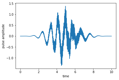
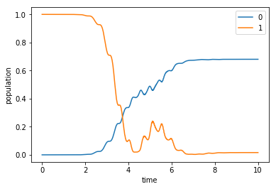
Simulate dynamics of the optimized pulse

We want to see how much the results have improved after the optimization.

plot_pulse(oct_result.optimized_controls[0], tlist)

opt_dynamics = [oct_result.optimized_objectives[x].mesolve(
    tlist, e_ops=[proj0, proj1]) for x in [0,1]]

opt_states = [oct_result.optimized_objectives[x].mesolve(tlist) for x in [0,1]]

plot_population(opt_dynamics[0])

plot_population(opt_dynamics[1])

In this case we do not only care about the expected value for the states, but since we want to implement a gate it is necessary to check whether we are performing a coherent control. We are then interested in the phase difference that we obtain after propagating the states from the logic basis.

def plot_gate(result):

    num = len(result[0].states)
    overlap_0 = np.vectorize(lambda i: np.angle(result[0].states[i].overlap(psi1)))
    overlap_1 = np.vectorize(lambda i: np.angle(result[1].states[i].overlap(psi0)))

    rel_phase = (overlap_0(np.arange(num))- overlap_1(np.arange(num)))%(2*np.pi)

    fig, ax = plt.subplots()
    ax.plot(result[0].times, rel_phase/np.pi)
    ax.set_xlabel('time')
    ax.set_ylabel('relative phase (π)')
    plt.show(fig)
    print('Final relative phase = %.2e' % rel_phase[-1])

plot_gate(opt_states)

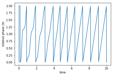
Final relative phase = 7.06e-02

We may also propagate the optimization result using the same propagator that was used in the optimization (instead of qutip.mesolve). The main difference between the two propagations is that mesolve assumes piecewise constant pulses that switch between two points in tlist, whereas propagate assumes that pulses are constant on the intervals of tlist, and thus switches on the points in tlist.

opt_dynamics2 = [oct_result.optimized_objectives[x].propagate(
    tlist, e_ops=[proj0, proj1], propagator=krotov.propagators.expm) for x in [0,1]]

The difference between the two propagations gives an indication of the “time discretization error”. If this error were unacceptably large, we would need a smaller time step.

"%.2e" % abs(opt_dynamics2[0].expect[1][-1] - opt_dynamics[0].expect[1][-1])

'1.40e-04'