Time Discretization Schemes

import numpy as np
import matplotlib.pylab as plt

There are some subtleties in how QuTiP discretizes controls versus the requirements of a gradient-based optimization. Understanding these subtleties is not critical for using this package (so you may skip this section of the documentation), but it is important for anyone trying to re-implement Krotov’s method in another language.

QuTiP, in its propagation routine mesolve, takes the controls to be exact at the values of the time grid (tlist), and piecewise-constant in the range ±dt/2 around each grid points. That is, controls switch at the midpoint between any two points in tlist.

In contrast, Krotov’s method (as well as any other gradient method, such as GRAPE) requires pulses to be constant on the intervals of the time grid, and switch on the time grid points. The implementation of Krotov’s method handles this transparently: On input and output, the controls in the Objectives follow the convention in QuTiP. Controls can be either functions that will be evaluated at the points in tlist, or an array of values of the same length as tlist.Internally, Krotov uses the control_onto_interval and pulse_onto_tlist to convert the control values to be constant on the intervals of the time grid (resulting in an array of pulse values that has one value less than the points in tlist), and back:

import krotov
from krotov.structural_conversions import pulse_onto_tlist, control_onto_interval

The names of these routines reflects a convention used in the implementation, where “controls” are defined on tlist, and “pulses” are defined on the intervals of tlist.

The transformation between the two is invertible. Since we generally care a lot about the boundaries of the controls (which often should be exactly zero), the initial and final value of the control is kept unchanged when converting to midpoints. For any other point, the “control” values at the time grid points will be the average of the “pulse” values of the intervals before and after that point on the time grid.

We can illustrate both sampling conventions in a plot:

def plot_sampling_points(func, N=30, T=10, peg='gridpoints'):
    """Show the numerical sampling for a control `func`

    Args:
        func (callable): Callable control ``func(t, None)`` for every point on
            the time grid
        N (int): number of points on the time grid
        T (float): final time
        peg (str): If 'midpoints', make the sampling exact at the
            midpoints of the time grid. If 'gridpoints', make the sampling
            exact at the points of the time grid.
    """
    tlist = np.linspace(0, T, N)
    dt = tlist[1] - tlist[0]
    tlist_midpoints = []
    for i in range(len(tlist) - 1):
        tlist_midpoints.append(0.5 * (tlist[i+1] + tlist[i]))
    tlist_midpoints = np.array(tlist_midpoints)
    tlist_exact = np.linspace(0, 10, 100)

    if peg == 'midpoints':
        pulse = np.array([func(t, None) for t in tlist_midpoints])
        control = pulse_onto_tlist(pulse)
    elif peg == 'gridpoints':
        control = np.array([func(t, None) for t in tlist])
        pulse = control_onto_interval(control)
    else:
        raise ValueError("Invalid peg")

    fig, ax = plt.subplots(figsize=(9, 7))
    ax.plot(
        tlist_exact, func(tlist_exact, None), '-', color='black',
        label='exact')
    ax.errorbar(
        tlist_midpoints, pulse, fmt='o', xerr=dt/2, color='blue',
        label="sampled on intervals")
    ax.errorbar(
        tlist, control, fmt='o', xerr=dt/2, color='red',
        label="sampled on time grid")
    ax.legend()
    ax.set_xlabel('time')
    ax.set_ylabel('pulse amplitude')
    plt.show(fig)

We’ll use a Blackman shape betwenn t=0 and T=10, as an example:

func = krotov.shapes.qutip_callback(krotov.shapes.blackman, t_start=0, t_stop=10)

If we did an optimization using that Blackman shape as a guess control, with N=10 time grid points, the sampling would look as follows:

plot_sampling_points(func, N=10, peg="gridpoints")

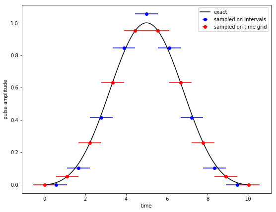
The red points indicate the sampling that QuTiP would use when propagating the guess control with mesolve. The blue points indicate the sampling that Krotov will use internally: each iteration yields an update for the blue points, and once the optimization finishes, the blue points are transformed back to the sampling of the red points.

An important detail is that if the guess controls are given as an (analytical) function, not an array, Krotov’s optimize_pulses will sample that function exactly onto tgrid before converting to the “guess pulses” defined on the midpoints. This is what was visualized above. If the controls were not discretized, but we were to choose the “pulses” based on the analytical formula, we would end up with the following sampling:

plot_sampling_points(func, N=10, peg="midpoints")

This exhibits a serious problem: After the transformation back to the sampling points on the time grid at the end of the optimization, it does not preserve the boundary values of the control to be zero at t=0 and t=T. Hence the choice to sample the control fields on input. Note that the same also applies to the shape function in the PulseOptions: these are also first sampled on the points of the time grid, and then converted to the interval representation, so that initial and final values of zero are preserved.

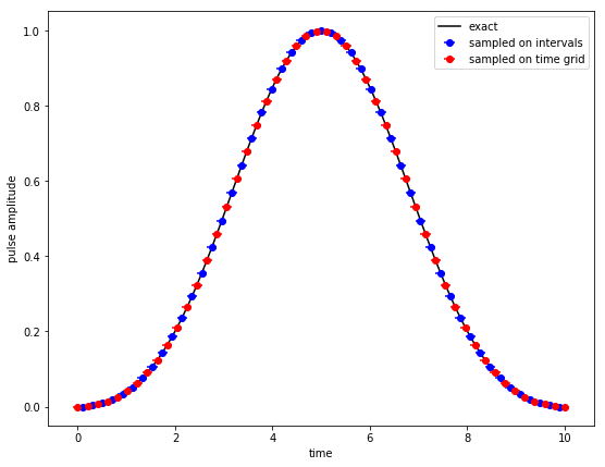
Obviously, when using just a few grid points as in the above plots, the result of a propagation may depend significantly on the sampling (the blue/red points can deviate significantly from the “exact” curve). This is the “discretization error”: In order for the optimization to be numerically useful, we must choose a time grid with a sufficiently small dt so that the difference between the two sampling choices becomes negligble:

plot_sampling_points(func, N=50, peg="gridpoints")

The Objective class has two methods mesolve and propagate that simulate the dynamics with the sampling on the grid points, and sampling on the intervals, respectively. You may compare the two to estimate the discretization error.

Bonus

If you run the notebook underlying this section of the documentation interactively (use the “launch binder” button at the top of the page), you may play around with your own choice of func and sampling points.

# NBVAL_SKIP
from ipywidgets import interact, interactive, fixed, interact_manual
import ipywidgets as widgets

%matplotlib notebook

interact(
    plot_sampling_points,
    N=widgets.IntSlider(min=5,max=100,step=5,value=10),
    T=fixed(10),
    peg=['gridpoints', 'midpoints'],
    func=fixed(func));