Optimization of a dissipative state-to-state transfer in a Lambda system

# NBVAL_IGNORE_OUTPUT
%load_ext watermark
import qutip
import numpy as np
import scipy
import matplotlib
import matplotlib.pylab as plt
import krotov
import qutip
from qutip import Qobj
import pickle
%watermark -v --iversions

qutip       4.3.1
numpy       1.15.4
scipy       1.1.0
matplotlib  3.0.2
matplotlib.pylab  1.15.4
krotov      0.0.1
CPython 3.6.7
IPython 7.2.0

\(\newcommand{tr}[0]{\operatorname{tr}} \newcommand{diag}[0]{\operatorname{diag}} \newcommand{abs}[0]{\operatorname{abs}} \newcommand{pop}[0]{\operatorname{pop}} \newcommand{aux}[0]{\text{aux}} \newcommand{opt}[0]{\text{opt}} \newcommand{tgt}[0]{\text{tgt}} \newcommand{init}[0]{\text{init}} \newcommand{lab}[0]{\text{lab}} \newcommand{rwa}[0]{\text{rwa}} \newcommand{bra}[1]{\langle#1\vert} \newcommand{ket}[1]{\vert#1\rangle} \newcommand{Bra}[1]{\left\langle#1\right\vert} \newcommand{Ket}[1]{\left\vert#1\right\rangle} \newcommand{Braket}[2]{\left\langle #1\vphantom{#2} \mid #2\vphantom{#1}\right\rangle} \newcommand{Ketbra}[2]{\left\vert#1\vphantom{#2} \right\rangle \hspace{-0.2em} \left\langle #2\vphantom{#1} \right\vert} \newcommand{op}[1]{\hat{#1}} \newcommand{Op}[1]{\hat{#1}} \newcommand{dd}[0]{\,\text{d}} \newcommand{Liouville}[0]{\mathcal{L}} \newcommand{DynMap}[0]{\mathcal{E}} \newcommand{identity}[0]{\mathbf{1}} \newcommand{Norm}[1]{\lVert#1\rVert} \newcommand{Abs}[1]{\left\vert#1\right\vert} \newcommand{avg}[1]{\langle#1\rangle} \newcommand{Avg}[1]{\left\langle#1\right\rangle} \newcommand{AbsSq}[1]{\left\vert#1\right\vert^2} \newcommand{Re}[0]{\operatorname{Re}} \newcommand{Im}[0]{\operatorname{Im}} \newcommand{toP}[0]{\omega_{12}} \newcommand{toS}[0]{\omega_{23}}\)

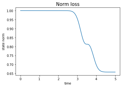
The aim of this example is to test the behaviour of Krotov’s algorithm when dealing with non-Hermitian Hamiltonians. This notebook is heavily based on the example “Optimization of a state-to-state transfer in a lambda system with RWA”, and therefore it is recommended that the reader become familiar with the system before hand. The main change in the results will be represented by the loss of norm during the propagation.

Define the Hamiltonian

We start with the usual 3-level lambda system such that \(E_1 < E_2\) and \(E_3 < E_2\). The states \(\Ket{1}\) and \(\Ket{2}\) are coupled coupled through a pump laser with frequency \(\omega_{P}=\omega_{P}(t)\) and similarly for the states \(\Ket{2}\) and \(\Ket{3}\) through a Stokes laser with frequency \(\omega_{S}=\omega_{S}(t)\).

The level \(\Ket{2}\) is assumed to experience a spontaneous decay into a reservoir that is out of the Hilbert space. This can be reproduced with a simple model that adds a dissipative coefficient \(\gamma > 0\), such that the original eigenvalue for the second level is modified into \(E_2 \rightarrow E_2 - i \gamma\).

We perform the same rotating wave approximation as described in the aforementioned example and obtain the time independent Hamiltonian

:nbsphinx-math:`begin{equation}

op{H}_{0} = Delta_{P}Ketbra{1}{1} -i

gamma Ketbra{2}{2} +Delta_{S} Ketbra{3}{3} end{equation}`

with the detunings \(\Delta_{P}=E_{1} + \omega_{P} - E_{2}\) and \(\Delta_{S} = E_{3} + \omega_{S} -E_{2}\).

The control Hamiltonian is again given by

:nbsphinx-math:`begin{equation} op{H}_{1}(t)

= op{H}_{1,P}(t) + op{H}_{1,S}(t) = Omega_{P}(t)

Ketbra{1}{2} +

Omega_{S}(t)Ketbra{2}{3} + text{H.c.},,

end{equation}` where \(\Omega_{P} = \Omega_{P}(t) = \frac{\mu_{21} \varepsilon_{P}(t)}{2} e^{-i\Phi_{S}(t) t}\) and \(\Omega_{S} = \Omega_{S}(t) = \frac{\mu_{23} \varepsilon_{S}(t)}{2} e^{-i\Phi_{P}(t) t}\) with the phases \(\Phi_{P}(t) = \toP - \omega_{P}(t)\) and \(\Phi_{S}(t) = \toS - \omega_{S}(t)\) and \(\mu_{ij}\) the \(ij^{\text{th}}\) dipole-transition moment.

For optimizing the complex pulses we once again separate them into their real and imaginary parts, i.e., \(\Omega_{P}(t) = \Omega_{P}^\text{Re}(t) + i\Omega_{P}^\text{Im}(t)\) and \(\Omega_{S}(t) = \Omega_{S}^\text{Re}(t) + i\Omega_{S}^\text{Im}(t)\), so we can optimize four real pulses.

def ham_and_states():
    """Lambda-system Hamiltonian"""
    E1 = 0.0
    E2 = 10.0
    E3 = 5.0
    ω_P = 9.5
    ω_S = 4.5
    gamma = 0.5
    Ω_init = 5.0
    H0 = Qobj(
        [
            [E1 + ω_P - E2, 0.0, 0.0],
            [0.0, -gamma * 1.0j, 0.0],
            [0.0, 0.0, E3 + ω_S - E2],
        ]
    )

    H1P_re = Qobj([[0.0, -1.0, 0.0], [-1.0, 0.0, 0.0], [0.0, 0.0, 0.0]])
    H1P_im = Qobj([[0.0, -1.0j, 0.0], [1.0j, 0.0, 0.0], [0.0, 0.0, 0.0]])
    ΩP_re = lambda t, args: Ω_init
    ΩP_im = lambda t, args: Ω_init

    H1S_re = Qobj([[0.0, 0.0, 0.0], [0.0, 0.0, 1.0], [0.0, 1.0, 0.0]])
    H1S_im = Qobj([[0.0, 0.0, 0.0], [0.0, 0.0, 1.0j], [0.0, -1.0j, 0.0]])
    ΩS_re = lambda t, args: Ω_init
    ΩS_im = lambda t, args: Ω_init

    """Initial and target states"""
    psi0 = qutip.Qobj(np.array([1.0, 0.0, 0.0]))
    psi1 = qutip.Qobj(np.array([0.0, 0.0, 1.0]))

    return (
        [
            H0,
            [H1P_re, ΩP_re],
            [H1P_im, ΩP_im],
            [H1S_re, ΩS_re],
            [H1S_im, ΩS_im],
        ],
        psi0,
        psi1,
    )


H, psi0, psi1 = ham_and_states()

We check whether our Hamiltonians are Hermitian:

print("H0 is Hermitian: " + str(H[0].isherm))
print("H1 is Hermitian: "+ str(
        H[1][0].isherm
    and H[2][0].isherm
    and H[3][0].isherm
    and H[4][0].isherm))

H0 is Hermitian: False
H1 is Hermitian: True

We introduce projectors for each of the three energy levels \(\op{P}_{i} = \Ketbra{i}{i}\)

proj1 = Qobj([[1.,0.,0.],[0.,0.,0.],[0.,0.,0.]])
proj2 = Qobj([[0.,0.,0.],[0.,1.,0.],[0.,0.,0.]])
proj3 = Qobj([[0.,0.,0.],[0.,0.,0.],[0.,0.,1.]])

Define the optimization target

It is necessary to create a time grid to work with. In this example we choose a time interval starting at \(t_0 = 0\) and ending at \(t_f = 5\) with \(n_t = 500\) equidistant time steps.

t0 = 0.
tf = 5.
nt = 500
tlist = np.linspace(t0, tf, nt)

We define the objective to be a state to state transfer from the initial state \(\Ket{\Psi_{\init}} = \Ket{1}\) into the final state \(\Ket{\Psi_{\tgt}} = \Ket{3}\) at the final time \(t_{f}\).

objectives = [ krotov.Objective(initial_state=psi0, target=psi1, H=H) ]

Initial guess shapes

“stimulated Raman adiabatic passage” (STIRAP) is a process in which population in \(\Ket{1}\) is transferred into \(\Ket{3}\) without having to pass through \(\Ket{2}\) (which could for instance be a rapidly decaying level). In order for this process to occur, a temporally finite Stokes pulse of sufficient amplitude driving the \(\Ket{2} \leftrightarrow \Ket{3}\) transition is applied first, whilst second pump pulse of similar intensity follows some time later such that the pulses still have a partial temporal overlap.

In order to demonstrate the Krotov’s optimization method however, we choose an initial guess consisting of two low intensity and real Blackman pulses which are temporally disjoint.

For the real components of the matrix elements, we supply our guess pulses shaped as Blackman window functions S(t,offset), with an offset ensuring that the two pulses don’t overlap. The imaginary components are coupled to pulses that are zero at all times.

def S(t,offset):
    """Shape envelope function for the field update"""
    return krotov.shapes.blackman(t,1.+offset,4.+offset)

def shape_field_real(eps,offset):
    """Applies the total pulse shape to the real part of a guess pulse"""
    field_shaped = lambda t, args: eps(t, args)*S(t,offset)
    return field_shaped

def shape_field_imag(eps,offset):
    """Initializes the imaginary parts of the guess pulses to zero"""
    field_shaped = lambda t, args: eps(t, args)*0.
    return field_shaped

H[1][1] = shape_field_real(H[1][1],1.)
H[2][1] = shape_field_imag(H[2][1],1.)
H[3][1] = shape_field_real(H[3][1],-1.)
H[4][1] = shape_field_imag(H[4][1],-1.)

We choose an appropriate update factor \(\lambda_{a}\) for the problem at hand and make sure Krotov considers pulses which start and end with zero amplitude.

def update_shape(t):
    """Scales the Krotov methods update of the pulse value at the time t"""
    return krotov.shapes.flattop(t,0.,5.,0.3,func='sinsq')

opt_lambda = 2.0
pulse_options = {
    H[1][1]: krotov.PulseOptions(lambda_a=opt_lambda, shape=update_shape),
    H[2][1]: krotov.PulseOptions(lambda_a=opt_lambda, shape=update_shape),
    H[3][1]: krotov.PulseOptions(lambda_a=opt_lambda, shape=update_shape),
    H[4][1]: krotov.PulseOptions(lambda_a=opt_lambda, shape=update_shape),
}

It is possible to keep track of the fidelity during optimization by printing it after every iteration:

def print_fidelity(**args):
    F_re = np.average(np.array(args['tau_vals']).real)
    print("   F = %f" % F_re)
    return F_re

Simulate dynamics of the guess field

def plot_pulse(pulse, tlist, plottitle=None):
    fig, ax = plt.subplots()
    if callable(pulse):
        pulse = np.array([pulse(t, args=None) for t in tlist])
    ax.plot(tlist, pulse)
    ax.set_xlabel('time')
    ax.set_ylabel('pulse amplitude')
    if(isinstance(plottitle, str)):
        ax.set_title(plottitle, fontsize = 15)
    plt.show(fig)

plot_pulse(H[1][1], tlist, plottitle='Re($\Omega_P$)')
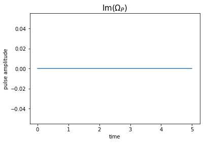
plot_pulse(H[2][1], tlist, plottitle='Im($\Omega_P$)')
plot_pulse(H[3][1], tlist, plottitle='Re($\Omega_S$)')
plot_pulse(H[4][1], tlist, plottitle='Im($\Omega_S$)')

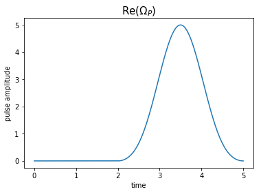
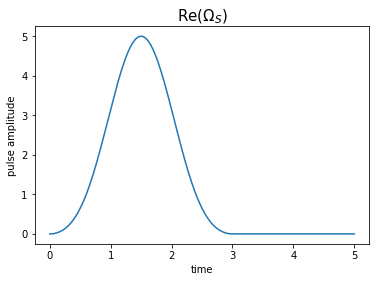
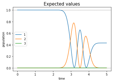
After assuring ourselves that our guess pulses appear as expected, we propagate the system using our guess. Since the pulses are temporally disjoint, we expect the first pulse to have no effect, whilst the second merely transfers population out of \(\Ket{1}\) into \(\Ket{2}\) and back again.

guess_dynamics = objectives[0].propagate(
    tlist, propagator=krotov.propagators.expm, e_ops=[proj1, proj2, proj3]
)
guess_states = objectives[0].propagate(
    tlist, propagator=krotov.propagators.expm
)

def plot_population(result):
    fig, ax = plt.subplots()
    ax.axhline(y=1.0, color='black', lw=0.5, ls='dashed')
    ax.axhline(y=0.0, color='black', lw=0.5, ls='dashed')
    ax.plot(result.times, result.expect[0], label='1')
    ax.plot(result.times, result.expect[1], label='2')
    ax.plot(result.times, result.expect[2], label='3')
    ax.legend()
    ax.set_title('Expected values', fontsize = 15)
    ax.set_xlabel('time')
    ax.set_ylabel('population')
    plt.show(fig)

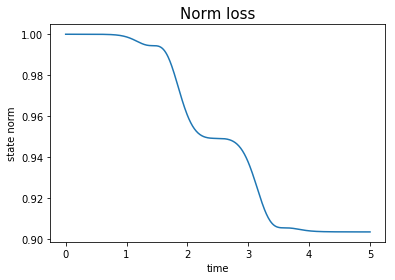
def plot_norm(result):

    state_norm = lambda i: result.states[i].norm()
    states_norm=np.vectorize(state_norm)

    fig, ax = plt.subplots()
    ax.plot(result.times, states_norm(np.arange(len(result.states))))
    ax.set_title('Norm loss', fontsize = 15)
    ax.set_xlabel('time')
    ax.set_ylabel('state norm')
    plt.show(fig)

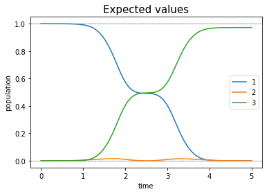
plot_population(guess_dynamics)
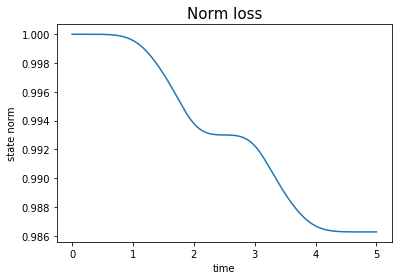
plot_norm(guess_states)

Optimize

We now use all the information that we have gathered to initialize the optimization routine. That is:

• The objectives: transferring population from \(\ket{1}\) to \(\ket{3}\) at \(t_f\).
• The pulse_options: initial pulses and their shapes restrictions.
• The propagator: in our example we will choose a simple matrix exponential.
• The chi_constructor: the optimization functional to use.
• The info_hook: all processes taking place inbetween iterations, for example printing the fidelity in each step.
• And the iter_stop: the number of iterations to perform the optimization.

oct_result = krotov.optimize_pulses(
    objectives, pulse_options, tlist,
    propagator=krotov.propagators.expm,
    chi_constructor=krotov.functionals.chis_re,
    info_hook=krotov.info_hooks.chain(
        #krotov.info_hooks.print_debug_information,
        print_fidelity),
    iter_stop=20
)

   F = -0.023471
   F = 0.252788
   F = 0.482934
   F = 0.645488
   F = 0.747822
   F = 0.808026
   F = 0.842348
   F = 0.861826
   F = 0.873076
   F = 0.879839
   F = 0.884167
   F = 0.887170
   F = 0.889446
   F = 0.891318
   F = 0.892959
   F = 0.894461
   F = 0.895876
   F = 0.897232
   F = 0.898543
   F = 0.899818
   F = 0.901063

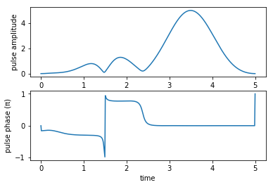
We can check that the algorithm takes into account the non Hermitian behaviour which leads to a non unitary final state. To improve the fidelity it is necessary to avoid these dissipative effects as much as possible.

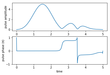
def plot_pulse_amplitude_and_phase(pulse_real, pulse_imaginary,tlist):
    ax1 = plt.subplot(211)
    ax2 = plt.subplot(212)
    amplitudes = [np.sqrt(x*x + y*y) for x,y in zip(pulse_real,pulse_imaginary)]
    phases = [np.arctan2(y,x)/np.pi for x,y in zip(pulse_real,pulse_imaginary)]
    ax1.plot(tlist,amplitudes)
    ax1.set_xlabel('time')
    ax1.set_ylabel('pulse amplitude')
    ax2.plot(tlist,phases)
    ax2.set_xlabel('time')
    ax2.set_ylabel('pulse phase (π)')
    plt.show()

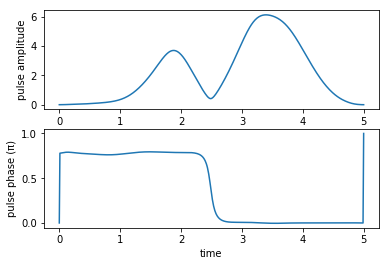
print("pump pulse amplitude and phase:")
plot_pulse_amplitude_and_phase(
    oct_result.optimized_controls[0], oct_result.optimized_controls[1], tlist)
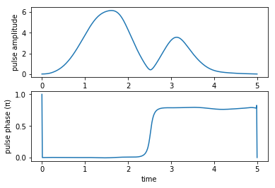
print("Stokes pulse amplitude and phase:")
plot_pulse_amplitude_and_phase(
    oct_result.optimized_controls[2], oct_result.optimized_controls[3], tlist)

pump pulse amplitude and phase:

Stokes pulse amplitude and phase:

We check the evolution of the population due to our optimized pulses.

opt_dynamics = oct_result.optimized_objectives[0].propagate(
    tlist, propagator=krotov.propagators.expm, e_ops=[proj1, proj2, proj3])
opt_states = oct_result.optimized_objectives[0].propagate(
    tlist, propagator=krotov.propagators.expm)

plot_population(opt_dynamics)
plot_norm(opt_states)

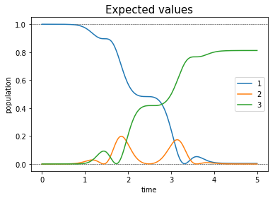
As we can see the algorithm takes into account the decay in level \(\ket{2}\) and minimizes the population in this level during the process.

However, convergence is relatively slow, and after 20 iterations, we have only achieved a 90% fidelity. As we can see from the population dynamics, we do not fully transfer the population in state \(\ket{3}\), and there is still non- negligible population in state \(\ket{2}\). If we were to continue up to iteration 2000, the optimization converges much farther:

oct_result = krotov.result.Result.load(
    './non_herm_oct_result.dump', objectives
)

print("Final fidelity: %.3f" % oct_result.info_vals[-1])

Final fidelity: 0.986

def plot_convergence(result):
    fig, ax = plt.subplots()
    ax.semilogy(result.iters, 1-np.array(result.info_vals))
    ax.set_xlabel('OCT iteration')
    ax.set_ylabel('error')
    plt.show(fig)

plot_convergence(oct_result)

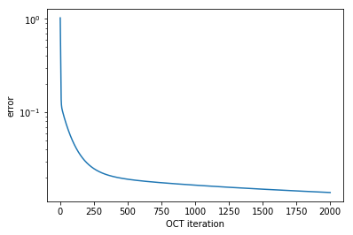
The dynamics now show a very good population transfer and negligible population in state \(\ket{2}\).

opt_dynamics = oct_result.optimized_objectives[0].propagate(
    tlist, propagator=krotov.propagators.expm, e_ops=[proj1, proj2, proj3])
opt_states = oct_result.optimized_objectives[0].propagate(
    tlist, propagator=krotov.propagators.expm)

print("pump pulse amplitude and phase:")
plot_pulse_amplitude_and_phase(
    oct_result.optimized_controls[0], oct_result.optimized_controls[1], tlist)
print("Stokes pulse amplitude and phase:")
plot_pulse_amplitude_and_phase(
    oct_result.optimized_controls[2], oct_result.optimized_controls[3], tlist)

pump pulse amplitude and phase:

Stokes pulse amplitude and phase:

plot_population(opt_dynamics)
plot_norm(opt_states)