![]()
![]()
Optimization of a State-to-State Transfer in a Two-Level-System
[1]:
# NBVAL_IGNORE_OUTPUT
%load_ext watermark
import qutip
import numpy as np
import scipy
import matplotlib
import matplotlib.pylab as plt
import krotov
%watermark -v --iversions
Python implementation: CPython
Python version       : 3.8.1
IPython version      : 7.24.1

qutip     : 4.6.1
matplotlib: 3.4.2
numpy     : 1.20.3
krotov    : 1.2.1+dev
scipy     : 1.6.3
\(\newcommand{tr}[0]{\operatorname{tr}} \newcommand{diag}[0]{\operatorname{diag}} \newcommand{abs}[0]{\operatorname{abs}} \newcommand{pop}[0]{\operatorname{pop}} \newcommand{aux}[0]{\text{aux}} \newcommand{opt}[0]{\text{opt}} \newcommand{tgt}[0]{\text{tgt}} \newcommand{init}[0]{\text{init}} \newcommand{lab}[0]{\text{lab}} \newcommand{rwa}[0]{\text{rwa}} \newcommand{bra}[1]{\langle#1\vert} \newcommand{ket}[1]{\vert#1\rangle} \newcommand{Bra}[1]{\left\langle#1\right\vert} \newcommand{Ket}[1]{\left\vert#1\right\rangle} \newcommand{Braket}[2]{\left\langle #1\vphantom{#2}\mid{#2}\vphantom{#1}\right\rangle} \newcommand{op}[1]{\hat{#1}} \newcommand{Op}[1]{\hat{#1}} \newcommand{dd}[0]{\,\text{d}} \newcommand{Liouville}[0]{\mathcal{L}} \newcommand{DynMap}[0]{\mathcal{E}} \newcommand{identity}[0]{\mathbf{1}} \newcommand{Norm}[1]{\lVert#1\rVert} \newcommand{Abs}[1]{\left\vert#1\right\vert} \newcommand{avg}[1]{\langle#1\rangle} \newcommand{Avg}[1]{\left\langle#1\right\rangle} \newcommand{AbsSq}[1]{\left\vert#1\right\vert^2} \newcommand{Re}[0]{\operatorname{Re}} \newcommand{Im}[0]{\operatorname{Im}}\)
This first example illustrates the basic use of the krotov package by solving a simple canonical optimization problem: the transfer of population in a two level system.
Two-level-Hamiltonian
We consider the Hamiltonian \(\op{H}_{0} = - \frac{\omega}{2} \op{\sigma}_{z}\), representing a simple qubit with energy level splitting \(\omega\) in the basis \(\{\ket{0},\ket{1}\}\). The control field \(\epsilon(t)\) is assumed to couple via the Hamiltonian \(\op{H}_{1}(t) = \epsilon(t) \op{\sigma}_{x}\) to the qubit, i.e., the control field effectively drives transitions between both qubit states.
[2]:
def hamiltonian(omega=1.0, ampl0=0.2):
    """Two-level-system Hamiltonian

    Args:
        omega (float): energy separation of the qubit levels
        ampl0 (float): constant amplitude of the driving field
    """
    H0 = -0.5 * omega * qutip.operators.sigmaz()
    H1 = qutip.operators.sigmax()

    def guess_control(t, args):
        return ampl0 * krotov.shapes.flattop(
            t, t_start=0, t_stop=5, t_rise=0.3, func="blackman"
        )

    return [H0, [H1, guess_control]]
[3]:
H = hamiltonian()
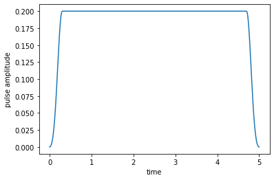
The control field here switches on from zero at \(t=0\) to it’s maximum amplitude 0.2 within the time period 0.3 (the switch-on shape is half a Blackman pulse). It switches off again in the time period 0.3 before the final time \(T=5\)). We use a time grid with 500 time steps between 0 and \(T\):
[4]:
tlist = np.linspace(0, 5, 500)
[5]:
def plot_pulse(pulse, tlist):
    fig, ax = plt.subplots()
    if callable(pulse):
        pulse = np.array([pulse(t, args=None) for t in tlist])
    ax.plot(tlist, pulse)
    ax.set_xlabel('time')
    ax.set_ylabel('pulse amplitude')
    plt.show(fig)
[6]:
plot_pulse(H[1][1], tlist)
Optimization target
The krotov package requires the goal of the optimization to be described by a list of Objective instances. In this example, there is only a single objective: the state-to-state transfer from initial state \(\ket{\Psi_{\init}} = \ket{0}\) to the target state \(\ket{\Psi_{\tgt}} = \ket{1}\), under the dynamics of the Hamiltonian \(\op{H}(t)\):
[7]:
objectives = [
    krotov.Objective(
        initial_state=qutip.ket("0"), target=qutip.ket("1"), H=H
    )
]

objectives
[7]:
[Objective[|Ψ₀(2)⟩ to |Ψ₁(2)⟩ via [H₀[2,2], [H₁[2,2], u₁(t)]]]]
In addition, we would like to maintain the property of the control field to be zero at \(t=0\) and \(t=T\), with a smooth switch-on and switch-off. We can define an “update shape” \(S(t) \in [0, 1]\) for this purpose: Krotov’s method will update the field at each point in time proportionally to \(S(t)\); wherever \(S(t)\) is zero, the optimization will not change the value of the control from the original guess.
[8]:
def S(t):
    """Shape function for the field update"""
    return krotov.shapes.flattop(
        t, t_start=0, t_stop=5, t_rise=0.3, t_fall=0.3, func='blackman'
    )
Beyond the shape, Krotov’s method uses a parameter \(\lambda_a\) for each control field that determines the overall magnitude of the respective field in each iteration (the smaller \(\lambda_a\), the larger the update; specifically, the update is proportional to \(\frac{S(t)}{\lambda_a}\)). Both the update-shape \(S(t)\) and the \(\lambda_a\) parameter must be passed to the optimization routine as “pulse options”:
[9]:
pulse_options = {
    H[1][1]: dict(lambda_a=5, update_shape=S)
}
Simulate dynamics under the guess field
Before running the optimization procedure, we first simulate the dynamics under the guess field \(\epsilon_{0}(t)\). The following solves equation of motion for the defined objective, which contains the initial state \(\ket{\Psi_{\init}}\) and the Hamiltonian \(\op{H}(t)\) defining its evolution. This delegates to QuTiP’s usual mesolve function.
We use the projectors \(\op{P}_0 = \ket{0}\bra{0}\) and \(\op{P}_1 = \ket{1}\bra{1}\) for calculating the population:
[10]:
proj0 = qutip.ket2dm(qutip.ket("0"))
proj1 = qutip.ket2dm(qutip.ket("1"))
[11]:
guess_dynamics = objectives[0].mesolve(tlist, e_ops=[proj0, proj1])
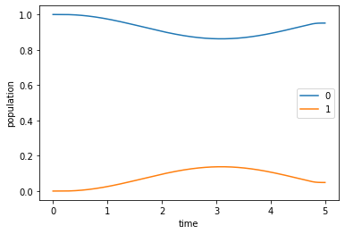
The plot of the population dynamics shows that the guess field does not transfer the initial state \(\ket{\Psi_{\init}} = \ket{0}\) to the desired target state \(\ket{\Psi_{\tgt}} = \ket{1}\) (so the optimization will have something to do).
[12]:
def plot_population(result):
    fig, ax = plt.subplots()
    ax.plot(result.times, result.expect[0], label='0')
    ax.plot(result.times, result.expect[1], label='1')
    ax.legend()
    ax.set_xlabel('time')
    ax.set_ylabel('population')
    plt.show(fig)
[13]:
plot_population(guess_dynamics)
Optimize
In the following we optimize the guess field \(\epsilon_{0}(t)\) such that the intended state-to-state transfer \(\ket{\Psi_{\init}} \rightarrow \ket{\Psi_{\tgt}}\) is solved, via the krotov package’s central optimize_pulses routine. It requires, besides the previously defined objectives, information about the optimization functional \(J_T\) (implicitly, via chi_constructor, which calculates the states \(\ket{\chi} = \frac{J_T}{\bra{\Psi}}\)).
Here, we choose \(J_T = J_{T,\text{ss}} = 1 - F_{\text{ss}}\) with \(F_{\text{ss}} = \Abs{\Braket{\Psi_{\tgt}}{\Psi(T)}}^2\), with \(\ket{\Psi(T)}\) the forward propagated state of \(\ket{\Psi_{\init}}\). Even though \(J_T\) is not explicitly required for the optimization, it is nonetheless useful to be able to calculate and print it as a way to provide some feedback about the optimization progress. Here, we pass as an info_hook the function
krotov.info_hooks.print_table, using krotov.functionals.J_T_ss (which implements the above functional; the krotov library contains implementations of all the “standard” functionals used in quantum control). This info_hook prints a tabular overview after each iteration, containing the value of \(J_T\), the magnitude of the integrated pulse update, and information on how much \(J_T\) (and the full Krotov functional \(J\)) changes between iterations. It also stores the
value of \(J_T\) internally in the Result.info_vals attribute.
The value of \(J_T\) can also be used to check the convergence. In this example, we limit the number of total iterations to 10, but more generally, we could use the check_convergence parameter to stop the optimization when \(J_T\) falls below some threshold. Here, we only pass a function that checks that the value of \(J_T\) is monotonically decreasing. The krotov.convergence.check_monotonic_error relies on krotov.info_hooks.print_table internally having stored the value
of \(J_T\) to the Result.info_vals in each iteration.
[14]:
opt_result = krotov.optimize_pulses(
    objectives,
    pulse_options=pulse_options,
    tlist=tlist,
    propagator=krotov.propagators.expm,
    chi_constructor=krotov.functionals.chis_ss,
    info_hook=krotov.info_hooks.print_table(J_T=krotov.functionals.J_T_ss),
    check_convergence=krotov.convergence.Or(
        krotov.convergence.value_below('1e-3', name='J_T'),
        krotov.convergence.check_monotonic_error,
    ),
    store_all_pulses=True,
)
iter.      J_T    ∫gₐ(t)dt          J       ΔJ_T         ΔJ  secs
0     9.51e-01    0.00e+00   9.51e-01        n/a        n/a     0
1     9.24e-01    1.20e-02   9.36e-01  -2.71e-02  -1.50e-02     1
2     8.83e-01    1.83e-02   9.02e-01  -4.11e-02  -2.28e-02     1
3     8.23e-01    2.71e-02   8.50e-01  -6.06e-02  -3.35e-02     1
4     7.37e-01    3.84e-02   7.76e-01  -8.52e-02  -4.68e-02     1
5     6.26e-01    5.07e-02   6.77e-01  -1.11e-01  -6.05e-02     1
6     4.96e-01    6.04e-02   5.56e-01  -1.31e-01  -7.02e-02     1
7     3.62e-01    6.30e-02   4.25e-01  -1.34e-01  -7.09e-02     1
8     2.44e-01    5.65e-02   3.00e-01  -1.18e-01  -6.15e-02     1
9     1.53e-01    4.39e-02   1.97e-01  -9.03e-02  -4.64e-02     1
10    9.20e-02    3.02e-02   1.22e-01  -6.14e-02  -3.12e-02     1
11    5.35e-02    1.90e-02   7.25e-02  -3.85e-02  -1.94e-02     1
12    3.06e-02    1.14e-02   4.20e-02  -2.29e-02  -1.15e-02     1
13    1.73e-02    6.60e-03   2.39e-02  -1.32e-02  -6.64e-03     1
14    9.78e-03    3.76e-03   1.35e-02  -7.54e-03  -3.78e-03     1
15    5.52e-03    2.13e-03   7.65e-03  -4.26e-03  -2.13e-03     1
16    3.11e-03    1.20e-03   4.31e-03  -2.40e-03  -1.20e-03     1
17    1.76e-03    6.77e-04   2.43e-03  -1.36e-03  -6.78e-04     1
18    9.91e-04    3.82e-04   1.37e-03  -7.64e-04  -3.82e-04     1
[15]:
opt_result
[15]:
Krotov Optimization Result
--------------------------
- Started at 2021-11-07 05:48:09
- Number of objectives: 1
- Number of iterations: 18
- Reason for termination: Reached convergence: J_T < 1e-3
- Ended at 2021-11-07 05:48:35 (0:00:26)
Simulate the dynamics under the optimized field
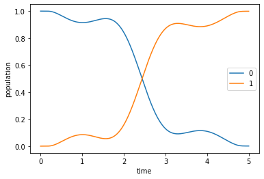
Having obtained the optimized control field, we can simulate the dynamics to verify that the optimized field indeed drives the initial state \(\ket{\Psi_{\init}} = \ket{0}\) to the desired target state \(\ket{\Psi_{\tgt}} = \ket{1}\).
[16]:
opt_dynamics = opt_result.optimized_objectives[0].mesolve(
    tlist, e_ops=[proj0, proj1])
[17]:
plot_population(opt_dynamics)
To gain some intuition on how the controls and the dynamics change throughout the optimization procedure, we can generate a plot of the control fields and the dynamics after each iteration of the optimization algorithm. This is possible because we set store_all_pulses=True in the call to optimize_pulses, which allows to recover the optimized controls from each iteration from Result.all_pulses. The flag is not set to True by default, as for long-running optimizations with thousands or
tens of thousands iterations, the storage of all control fields may require significant memory.
[18]:
def plot_iterations(opt_result):
    """Plot the control fields in population dynamics over all iterations.

    This depends on ``store_all_pulses=True`` in the call to
    `optimize_pulses`.
    """
    fig, [ax_ctr, ax_dyn] = plt.subplots(nrows=2, figsize=(8, 10))
    n_iters = len(opt_result.iters)
    for (iteration, pulses) in zip(opt_result.iters, opt_result.all_pulses):
        controls = [
            krotov.conversions.pulse_onto_tlist(pulse)
            for pulse in pulses
        ]
        objectives = opt_result.objectives_with_controls(controls)
        dynamics = objectives[0].mesolve(
            opt_result.tlist, e_ops=[proj0, proj1]
        )
        if iteration == 0:
            ls = '--'  # dashed
            alpha = 1  # full opacity
            ctr_label = 'guess'
            pop_labels = ['0 (guess)', '1 (guess)']
        elif iteration == opt_result.iters[-1]:
            ls = '-'  # solid
            alpha = 1  # full opacity
            ctr_label = 'optimized'
            pop_labels = ['0 (optimized)', '1 (optimized)']
        else:
            ls = '-'  # solid
            alpha = 0.5 * float(iteration) / float(n_iters)  # max 50%
            ctr_label = None
            pop_labels = [None, None]
        ax_ctr.plot(
            dynamics.times,
            controls[0],
            label=ctr_label,
            color='black',
            ls=ls,
            alpha=alpha,
        )
        ax_dyn.plot(
            dynamics.times,
            dynamics.expect[0],
            label=pop_labels[0],
            color='#1f77b4',  # default blue
            ls=ls,
            alpha=alpha,
        )
        ax_dyn.plot(
            dynamics.times,
            dynamics.expect[1],
            label=pop_labels[1],
            color='#ff7f0e',  # default orange
            ls=ls,
            alpha=alpha,
        )
    ax_dyn.legend()
    ax_dyn.set_xlabel('time')
    ax_dyn.set_ylabel('population')
    ax_ctr.legend()
    ax_ctr.set_xlabel('time')
    ax_ctr.set_ylabel('control amplitude')
    plt.show(fig)
[19]:
plot_iterations(opt_result)
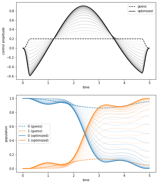
The initial guess (dashed) and final optimized (solid) control amplitude and resulting dynamics are shown with full opacity, whereas the curves corresponding intermediate iterations are shown with decreasing transparency.