![]()
![]()
Optimization towards a Perfect Entangler
[1]:
# NBVAL_IGNORE_OUTPUT
%load_ext watermark
import qutip
import numpy as np
import scipy
import matplotlib
import matplotlib.pylab as plt
import krotov
from IPython.display import display
import weylchamber as wc
from weylchamber.visualize import WeylChamber
from weylchamber.coordinates import from_magic

%watermark -v --iversions
Python implementation: CPython
Python version       : 3.8.1
IPython version      : 7.24.1

scipy      : 1.6.3
qutip      : 4.6.1
weylchamber: 0.3.2
matplotlib : 3.4.2
krotov     : 1.2.1+dev
numpy      : 1.20.3
\(\newcommand{tr}[0]{\operatorname{tr}} \newcommand{diag}[0]{\operatorname{diag}} \newcommand{abs}[0]{\operatorname{abs}} \newcommand{pop}[0]{\operatorname{pop}} \newcommand{aux}[0]{\text{aux}} \newcommand{opt}[0]{\text{opt}} \newcommand{tgt}[0]{\text{tgt}} \newcommand{init}[0]{\text{init}} \newcommand{lab}[0]{\text{lab}} \newcommand{rwa}[0]{\text{rwa}} \newcommand{bra}[1]{\langle#1\vert} \newcommand{ket}[1]{\vert#1\rangle} \newcommand{Bra}[1]{\left\langle#1\right\vert} \newcommand{Ket}[1]{\left\vert#1\right\rangle} \newcommand{Braket}[2]{\left\langle #1\vphantom{#2} \mid #2\vphantom{#1}\right\rangle} \newcommand{op}[1]{\hat{#1}} \newcommand{Op}[1]{\hat{#1}} \newcommand{dd}[0]{\,\text{d}} \newcommand{Liouville}[0]{\mathcal{L}} \newcommand{DynMap}[0]{\mathcal{E}} \newcommand{identity}[0]{\mathbf{1}} \newcommand{Norm}[1]{\lVert#1\rVert} \newcommand{Abs}[1]{\left\vert#1\right\vert} \newcommand{avg}[1]{\langle#1\rangle} \newcommand{Avg}[1]{\left\langle#1\right\rangle} \newcommand{AbsSq}[1]{\left\vert#1\right\vert^2} \newcommand{Re}[0]{\operatorname{Re}} \newcommand{Im}[0]{\operatorname{Im}}\)
This example demonstrates the optimization with an “unconventional” optimization target. Instead of a state-to-state transition, or the realization of a specific quantum gate, we optimize for an arbitrary perfectly entangling gate. See
Watts, et al., Phys. Rev. A 91, 062306 (2015)
Goerz, et al., Phys. Rev. A 91, 062307 (2015)
for details.
Hamiltonian
We consider a generic two-qubit Hamiltonian (motivated from the example of two superconducting transmon qubits, truncated to the logical subspace),
where \(\omega_1\) and \(\omega_2\) are the energy level splitting of the respective qubit, \(J\) is the effective coupling strength and \(u(t)\) is the control field. \(\lambda\) defines the strength of the qubit-control coupling for qubit 2, relative to qubit 1.
We use the following parameters:
[2]:
w1 = 1.1  # qubit 1 level splitting
w2 = 2.1  # qubit 2 level splitting
J = 0.2  # effective qubit coupling
u0 = 0.3  # initial driving strength
la = 1.1  # relative pulse coupling strength of second qubit
T = 25.0  # final time
nt = 250  # number of time steps

tlist = np.linspace(0, T, nt)
These are for illustrative purposes only, and do not correspond to any particular physical system.
The initial guess is defined as
[3]:
def eps0(t, args):
    return u0 * krotov.shapes.flattop(
        t, t_start=0, t_stop=T, t_rise=(T / 20), t_fall=(T / 20), func='sinsq'
    )
[4]:
def plot_pulse(pulse, tlist):
    fig, ax = plt.subplots()
    if callable(pulse):
        pulse = np.array([pulse(t, args=None) for t in tlist])
    ax.plot(tlist, pulse)
    ax.set_xlabel('time')
    ax.set_ylabel('pulse amplitude')
    plt.show(fig)
[5]:
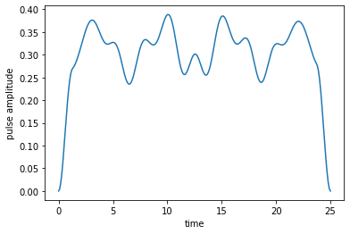
plot_pulse(eps0, tlist)
We instantiate the Hamiltonian with this guess pulse
[6]:
def hamiltonian(w1=w1, w2=w2, J=J, la=la, u0=u0):
    """Two qubit Hamiltonian

    Args:
        w1 (float): energy separation of the first qubit levels
        w2 (float): energy separation of the second qubit levels
        J (float): effective coupling between both qubits
        la (float): factor that pulse coupling strength differs for second qubit
        u0 (float): constant amplitude of the driving field
    """
    # local qubit Hamiltonians
    Hq1 = 0.5 * w1 * np.diag([-1, 1])
    Hq2 = 0.5 * w2 * np.diag([-1, 1])

    # lift Hamiltonians to joint system operators
    H0 = np.kron(Hq1, np.identity(2)) + np.kron(np.identity(2), Hq2)

    # define the interaction Hamiltonian
    sig_x = np.array([[0, 1], [1, 0]])
    sig_y = np.array([[0, -1j], [1j, 0]])
    Hint = 2 * J * (np.kron(sig_x, sig_x) + np.kron(sig_y, sig_y))
    H0 = H0 + Hint

    # define the drive Hamiltonian
    H1 = np.kron(np.array([[0, 1], [1, 0]]), np.identity(2)) + la * np.kron(
        np.identity(2), np.array([[0, 1], [1, 0]])
    )

    # convert Hamiltonians to QuTiP objects
    H0 = qutip.Qobj(H0)
    H1 = qutip.Qobj(H1)

    return [H0, [H1, eps0]]


H = hamiltonian(w1=w1, w2=w2, J=J, la=la, u0=u0)
As well as the canonical two-qubit logical basis,
[7]:
psi_00 = qutip.Qobj(np.kron(np.array([1, 0]), np.array([1, 0])))
psi_01 = qutip.Qobj(np.kron(np.array([1, 0]), np.array([0, 1])))
psi_10 = qutip.Qobj(np.kron(np.array([0, 1]), np.array([1, 0])))
psi_11 = qutip.Qobj(np.kron(np.array([0, 1]), np.array([0, 1])))
with the corresponding projectors to calculate population dynamics below.
[8]:
proj_00 = qutip.ket2dm(psi_00)
proj_01 = qutip.ket2dm(psi_01)
proj_10 = qutip.ket2dm(psi_10)
proj_11 = qutip.ket2dm(psi_11)
Objectives for a perfect entangler
Our optimization target is the closest perfectly entangling gate, quantified by the perfect-entangler functional
where \(g_1, g_2, g_3\) are the local invariants of the implemented gate that uniquely identify its non-local content. The local invariants are closely related to the Weyl coordinates \(c_1, c_2, c_3\), which provide a useful geometric visualization in the Weyl chamber. The perfectly entangling gates lie within a polyhedron in the Weyl chamber and \(F_{PE}\) becomes zero at its boundaries. We define \(F_{PE} \equiv 0\) for all perfect entanglers (inside the polyhedron)
A list of four objectives that encode the minimization of \(F_{PE}\) are generated by calling the gate_objectives function with the canonical basis, and "PE" as target “gate”.
[9]:
objectives = krotov.gate_objectives(
    basis_states=[psi_00, psi_01, psi_10, psi_11], gate="PE", H=H
)
[10]:
objectives
[10]:
[Objective[|Ψ₀(4)⟩ to PE via [H₀[4,4], [H₁[4,4], u₁(t)]]],
 Objective[|Ψ₁(4)⟩ to PE via [H₀[4,4], [H₁[4,4], u₁(t)]]],
 Objective[|Ψ₂(4)⟩ to PE via [H₀[4,4], [H₁[4,4], u₁(t)]]],
 Objective[|Ψ₃(4)⟩ to PE via [H₀[4,4], [H₁[4,4], u₁(t)]]]]
The initial states in these objectives are not the canonical basis states, but a Bell basis,
[11]:
# NBVAL_IGNORE_OUTPUT
for obj in objectives:
    display(obj.initial_state)
Since we don’t know which perfect entangler the optimization result will implement, we cannot associate any “target state” with each objective, and the target attribute is set to the string ‘PE’.
We can treat the above objectives as a “black box”; the only important consideration is that the chi_constructor that we will pass to optimize_pulses to calculating the boundary condition for the backwards propagation,
must be consistent with how the objectives are set up. For the perfect entanglers functional, the calculation of the \(\ket{\chi_{k}}\) is relatively complicated. The weylchamber package (https://github.com/qucontrol/weylchamber) contains a suitable routine that works on the objectives exactly as defined above (specifically, under the assumption that the \(\ket{\phi_k}\) are the appropriate Bell states):
[12]:
help(wc.perfect_entanglers.make_PE_krotov_chi_constructor)
Help on function make_PE_krotov_chi_constructor in module weylchamber.perfect_entanglers:

make_PE_krotov_chi_constructor(canonical_basis, unitarity_weight=0)
    Return a constructor for the χ's in a PE optimization.

    Return a `chi_constructor` that determines the boundary condition of the
    backwards propagation in an optimization towards a perfect entangler in
    Krotov's method, based on the foward-propagtion of the Bell states. In
    detail, the function returns a callable function that calculates

    .. math::

        \ket{\chi_{i}}
        =
        \frac{\partial F_{PE}}{\partial \bra{\phi_i}}
        \Bigg|_{\ket{\phi_{i}(T)}}

    for all $i$ with $\ket{\phi_{0}(T)}, ..., \ket{\phi_{3}(T)}$ the forward
    propagated Bell states at final time $T$, cf. Eq. (33b) in Ref. [1].
    $F_{PE}$ is the perfect-entangler functional
    :func:`~weylchamber.perfect_entanglers.F_PE`. For the details of the
    derivative see Appendix G in Ref. [2].

    References:

    [1] `M. H. Goerz, et al., Phys. Rev. A 91, 062307 (2015)
    <https://doi.org/10.1103/PhysRevA.91.062307>`_

    [2] `M. H. Goerz, Optimizing Robust Quantum Gates in Open Quantum Systems.
    PhD thesis, University of Kassel, 2015
    <https://michaelgoerz.net/research/diss_goerz.pdf>`_

    Args:
        canonical_basis (list[qutip.Qobj]): A list of four basis states that
            define the canonical basis $\ket{00}$, $\ket{01}$, $\ket{10}$, and
            $\ket{11}$ of the logical subspace.
        unitarity_weight (float): A weight in [0, 1] that determines how much
            emphasis is placed on  maintaining population in the logical
            subspace.

    Returns:
        callable: a function ``chi_constructor(fw_states_T, **kwargs)`` that
        receives the result of a foward propagation of the Bell states
        (obtained from `canonical_basis` via
        :func:`weylchamber.gates.bell_basis`), and returns a list of statex
        $\ket{\chi_{i}}$ that are the boundary condition for the backward
        propagation in Krotov's method. Positional arguments beyond
        `fw_states_T` are ignored.
[13]:
chi_constructor = wc.perfect_entanglers.make_PE_krotov_chi_constructor(
    [psi_00, psi_01, psi_10, psi_11]
)
Again, the key point to take from this is that when defining a new or unusual functional, the ``chi_constructor`` must be congruent with the way the objectives are defined. As a user, you can choose whatever definition of objectives and implementation of chi_constructor is most suitable, as long they are compatible.
Second Order Update Equation
As the perfect-entangler functional \(F_{PE}\) is non-linear in the states, Krotov’s method requires the second-order contribution in order to guarantee monotonic convergence (see D. M. Reich, et al., J. Chem. Phys. 136, 104103 (2012) for details). The second order update equation reads
where the term proportional to \(\sigma(t)\) defines the second-order contribution. In order to use the second-order term, we need to pass a function to evaluate this \(\sigma(t)\) as sigma to optimize_pulses. We use the equation
with \(\varepsilon_A\) a small non-negative number, and \(A\) a parameter that can be recalculated numerically after each iteration (see D. M. Reich, et al., J. Chem. Phys. 136, 104103 (2012) for details).
Generally, \(\sigma(t)\) has parametric dependencies like \(A\) in this example, which should be refreshed for each iteration. Thus, since sigma holds internal state, it must be implemented as an object subclassing from krotov.second_order.Sigma:
[14]:
class sigma(krotov.second_order.Sigma):
    def __init__(self, A, epsA=0):
        self.A = A
        self.epsA = epsA

    def __call__(self, t):
        ϵ, A = self.epsA, self.A
        return -max(ϵ, 2 * A + ϵ)

    def refresh(
        self,
        forward_states,
        forward_states0,
        chi_states,
        chi_norms,
        optimized_pulses,
        guess_pulses,
        objectives,
        result,
    ):
        try:
            Delta_J_T = result.info_vals[-1][0] - result.info_vals[-2][0]
        except IndexError:  # first iteration
            Delta_J_T = 0
        self.A = krotov.second_order.numerical_estimate_A(
            forward_states, forward_states0, chi_states, chi_norms, Delta_J_T
        )
This combines the evaluation of the function, sigma(t), with the recalculation of \(A\) (or whatever parametrizations another \(\sigma(t)\) function might contain) in sigma.refresh, which optimize_pulses invokes automatically at the end of each iteration.
Optimization
Before running the optimization, we define the shape function \(S(t)\) to maintain the smooth switch-on and switch-off, and the \(\lambda_a\) parameter that determines the overall magnitude of the pulse update in each iteration:
[15]:
def S(t):
    """Shape function for the field update"""
    return krotov.shapes.flattop(
        t, t_start=0, t_stop=T, t_rise=T / 20, t_fall=T / 20, func='sinsq'
    )

pulse_options = {H[1][1]: dict(lambda_a=1.0e2, update_shape=S)}
In previous examples, we have used info_hook routines that display and store the value of the functional \(J_T\). Here, we will also want to analyze the optimization in terms of the Weyl chamber coordinates \((c_1, c_2, c_3)\). We therefore write a custom print_fidelity routine that prints \(F_{PE}\) as well as the gate concurrence (as an alternative measure for the entangling power of quantum gates), and results in the storage of a nested tuple (F_PE, (c1, c2, c3)) for
each iteration, in Result.info_vals.
[16]:
def print_fidelity(**args):
    basis = [objectives[i].initial_state for i in [0, 1, 2, 3]]
    states = [args['fw_states_T'][i] for i in [0, 1, 2, 3]]
    U = wc.gates.gate(basis, states)
    c1, c2, c3 = wc.coordinates.c1c2c3(from_magic(U))
    g1, g2, g3 = wc.local_invariants.g1g2g3_from_c1c2c3(c1, c2, c3)
    conc = wc.perfect_entanglers.concurrence(c1, c2, c3)
    F_PE = wc.perfect_entanglers.F_PE(g1, g2, g3)
    print("    F_PE: %f\n    gate conc.: %f" % (F_PE, conc))
    return F_PE, [c1, c2, c3]
This structure must be taken into account in a check_convergence routine. This would affect routines like krotov.convergence.value_below that assume that Result.info_vals contains the values of \(J_T\) only. Here, we define a check that stops the optimization as soon as we reach a perfect entangler:
[17]:
def check_PE(result):
    # extract F_PE from (F_PE, [c1, c2, c3])
    F_PE = result.info_vals[-1][0]
    if F_PE <= 0:
        return "achieved perfect entangler"
    else:
        return None
[18]:
opt_result = krotov.optimize_pulses(
    objectives,
    pulse_options=pulse_options,
    tlist=tlist,
    propagator=krotov.propagators.expm,
    chi_constructor=chi_constructor,
    info_hook=krotov.info_hooks.chain(
        krotov.info_hooks.print_debug_information, print_fidelity
    ),
    check_convergence=check_PE,
    sigma=sigma(A=0.0),
    iter_stop=20,
)
Iteration 0
    objectives:
        1:|Ψ₀(4)⟩ to PE via [H₀[4,4], [H₁[4,4], u₁(t)]]
        2:|Ψ₁(4)⟩ to PE via [H₀[4,4], [H₁[4,4], u₁(t)]]
        3:|Ψ₂(4)⟩ to PE via [H₀[4,4], [H₁[4,4], u₁(t)]]
        4:|Ψ₃(4)⟩ to PE via [H₀[4,4], [H₁[4,4], u₁(t)]]
    adjoint objectives:
        1:⟨Ψ₀(4)| to PE via [H₂[4,4], [H₃[4,4], u₁(t)]]
        2:⟨Ψ₁(4)| to PE via [H₄[4,4], [H₅[4,4], u₁(t)]]
        3:⟨Ψ₂(4)| to PE via [H₆[4,4], [H₇[4,4], u₁(t)]]
        4:⟨Ψ₃(4)| to PE via [H₈[4,4], [H₉[4,4], u₁(t)]]
    propagator: expm
    chi_constructor: chi_constructor
    mu: derivative_wrt_pulse
    sigma: sigma
    S(t) (ranges): [0.000000, 1.000000]
    iter_start: 0
    iter_stop: 20
    duration: 1.5 secs (started at 2021-11-07 05:56:40)
    optimized pulses (ranges): [0.00, 0.30]
    ∫gₐ(t)dt: 0.00e+00
    λₐ: 1.00e+02
    storage (bw, fw, fw0): None, [4 * ndarray(250)] (0.5 MB), [4 * ndarray(250)] (0.5 MB)
    fw_states_T norm: 1.000000, 1.000000, 1.000000, 1.000000
    F_PE: 1.447335
    gate conc.: 0.479492
Iteration 1
    duration: 3.7 secs (started at 2021-11-07 05:56:42)
    optimized pulses (ranges): [0.00, 0.32]
    ∫gₐ(t)dt: 2.58e-01
    λₐ: 1.00e+02
    storage (bw, fw, fw0): [4 * ndarray(250)] (0.5 MB), [4 * ndarray(250)] (0.5 MB), [4 * ndarray(250)] (0.5 MB)
    fw_states_T norm: 1.000000, 1.000000, 1.000000, 1.000000
    F_PE: 0.998102
    gate conc.: 0.645579
Iteration 2
    duration: 3.7 secs (started at 2021-11-07 05:56:46)
    optimized pulses (ranges): [0.00, 0.34]
    ∫gₐ(t)dt: 2.20e-01
    λₐ: 1.00e+02
    storage (bw, fw, fw0): [4 * ndarray(250)] (0.5 MB), [4 * ndarray(250)] (0.5 MB), [4 * ndarray(250)] (0.5 MB)
    fw_states_T norm: 1.000000, 1.000000, 1.000000, 1.000000
    F_PE: 0.582566
    gate conc.: 0.784635
Iteration 3
    duration: 3.7 secs (started at 2021-11-07 05:56:49)
    optimized pulses (ranges): [0.00, 0.35]
    ∫gₐ(t)dt: 1.46e-01
    λₐ: 1.00e+02
    storage (bw, fw, fw0): [4 * ndarray(250)] (0.5 MB), [4 * ndarray(250)] (0.5 MB), [4 * ndarray(250)] (0.5 MB)
    fw_states_T norm: 1.000000, 1.000000, 1.000000, 1.000000
    F_PE: 0.304191
    gate conc.: 0.892999
Iteration 4
    duration: 3.7 secs (started at 2021-11-07 05:56:53)
    optimized pulses (ranges): [0.00, 0.37]
    ∫gₐ(t)dt: 7.72e-02
    λₐ: 1.00e+02
    storage (bw, fw, fw0): [4 * ndarray(250)] (0.5 MB), [4 * ndarray(250)] (0.5 MB), [4 * ndarray(250)] (0.5 MB)
    fw_states_T norm: 1.000000, 1.000000, 1.000000, 1.000000
    F_PE: 0.153498
    gate conc.: 0.951891
Iteration 5
    duration: 3.7 secs (started at 2021-11-07 05:56:57)
    optimized pulses (ranges): [0.00, 0.37]
    ∫gₐ(t)dt: 3.88e-02
    λₐ: 1.00e+02
    storage (bw, fw, fw0): [4 * ndarray(250)] (0.5 MB), [4 * ndarray(250)] (0.5 MB), [4 * ndarray(250)] (0.5 MB)
    fw_states_T norm: 1.000000, 1.000000, 1.000000, 1.000000
    F_PE: 0.076100
    gate conc.: 0.980700
Iteration 6
    duration: 3.7 secs (started at 2021-11-07 05:57:00)
    optimized pulses (ranges): [0.00, 0.38]
    ∫gₐ(t)dt: 2.03e-02
    λₐ: 1.00e+02
    storage (bw, fw, fw0): [4 * ndarray(250)] (0.5 MB), [4 * ndarray(250)] (0.5 MB), [4 * ndarray(250)] (0.5 MB)
    fw_states_T norm: 1.000000, 1.000000, 1.000000, 1.000000
    F_PE: 0.035062
    gate conc.: 0.993840
Iteration 7
    duration: 3.7 secs (started at 2021-11-07 05:57:04)
    optimized pulses (ranges): [0.00, 0.39]
    ∫gₐ(t)dt: 1.13e-02
    λₐ: 1.00e+02
    storage (bw, fw, fw0): [4 * ndarray(250)] (0.5 MB), [4 * ndarray(250)] (0.5 MB), [4 * ndarray(250)] (0.5 MB)
    fw_states_T norm: 1.000000, 1.000000, 1.000000, 1.000000
    F_PE: 0.012118
    gate conc.: 0.998971
Iteration 8
    duration: 3.7 secs (started at 2021-11-07 05:57:08)
    optimized pulses (ranges): [0.00, 0.39]
    ∫gₐ(t)dt: 6.68e-03
    λₐ: 1.00e+02
    storage (bw, fw, fw0): [4 * ndarray(250)] (0.5 MB), [4 * ndarray(250)] (0.5 MB), [4 * ndarray(250)] (0.5 MB)
    fw_states_T norm: 1.000000, 1.000000, 1.000000, 1.000000
    F_PE: -0.001422
    gate conc.: 1.000000
[19]:
opt_result
[19]:
Krotov Optimization Result
--------------------------
- Started at 2021-11-07 05:56:40
- Number of objectives: 4
- Number of iterations: 8
- Reason for termination: Reached convergence: achieved perfect entangler
- Ended at 2021-11-07 05:57:11 (0:00:31)
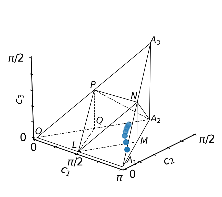
We can visualize how each iteration of the optimization brings the dynamics closer to the polyhedron of perfect entanglers (using the Weyl chamber coordinates that we calculated in the info_hook routine print_fidelity, and that were stored in Result.info_vals).
[20]:
w = WeylChamber()
c1c2c3 = [opt_result.info_vals[i][1] for i in range(len(opt_result.iters))]
for i in range(len(opt_result.iters)):
    w.add_point(c1c2c3[i][0], c1c2c3[i][1], c1c2c3[i][2])
w.plot()
/home/mgoerz/Documents/krotov/.tox/py38/lib/python3.8/site-packages/weylchamber/visualize.py:318: UserWarning: FixedFormatter should only be used together with FixedLocator
  ax.set_yticklabels(['0', '', '', '', '', r'$\pi/2$'])
/home/mgoerz/Documents/krotov/.tox/py38/lib/python3.8/site-packages/weylchamber/visualize.py:319: UserWarning: FixedFormatter should only be used together with FixedLocator
  ax.set_zticklabels(['0', '', '', '', '', r'$\pi/2$'])
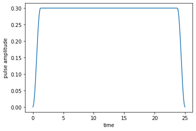
The final optimized control field looks like this:
[21]:
plot_pulse(opt_result.optimized_controls[0], tlist)