![]()
![]()
Optimization of a state-to-state transfer in a lambda system with RWA
[1]:
# NBVAL_IGNORE_OUTPUT
%load_ext watermark
import numpy as np
import scipy
import matplotlib
import matplotlib.pylab as plt
import krotov
import qutip
from qutip import Qobj
%watermark -v --iversions
qutip            4.3.1
krotov           0.3.0
matplotlib       3.0.3
scipy            1.2.1
numpy            1.15.4
matplotlib.pylab 1.15.4
CPython 3.6.8
IPython 7.3.0
\(\newcommand{tr}[0]{\operatorname{tr}} \newcommand{diag}[0]{\operatorname{diag}} \newcommand{abs}[0]{\operatorname{abs}} \newcommand{pop}[0]{\operatorname{pop}} \newcommand{aux}[0]{\text{aux}} \newcommand{opt}[0]{\text{opt}} \newcommand{tgt}[0]{\text{tgt}} \newcommand{init}[0]{\text{init}} \newcommand{lab}[0]{\text{lab}} \newcommand{rwa}[0]{\text{rwa}} \newcommand{bra}[1]{\langle#1\vert} \newcommand{ket}[1]{\vert#1\rangle} \newcommand{Bra}[1]{\left\langle#1\right\vert} \newcommand{Ket}[1]{\left\vert#1\right\rangle} \newcommand{Braket}[2]{\left\langle #1\vphantom{#2} \mid #2\vphantom{#1}\right\rangle} \newcommand{Ketbra}[2]{\left\vert#1\vphantom{#2} \right\rangle \hspace{-0.2em} \left\langle #2\vphantom{#1}\right\vert} \newcommand{op}[1]{\hat{#1}} \newcommand{Op}[1]{\hat{#1}} \newcommand{dd}[0]{\,\text{d}} \newcommand{Liouville}[0]{\mathcal{L}} \newcommand{DynMap}[0]{\mathcal{E}} \newcommand{identity}[0]{\mathbf{1}} \newcommand{Norm}[1]{\lVert#1\rVert} \newcommand{Abs}[1]{\left\vert#1\right\vert} \newcommand{avg}[1]{\langle#1\rangle} \newcommand{Avg}[1]{\left\langle#1\right\rangle} \newcommand{AbsSq}[1]{\left\vert#1\right\vert^2} \newcommand{Re}[0]{\operatorname{Re}} \newcommand{Im}[0]{\operatorname{Im}} \newcommand{toP}[0]{\omega_{12}} \newcommand{toS}[0]{\omega_{23}} \newcommand{oft}[0]{\left(t\right)}\)
The purpose of this example is to illustrate and test the use of complex control fields. Essentially, this is accomplished by rewriting the Hamiltonian as the sum of two independent controls (real and imaginary parts).
Define the Hamiltonian
The system consists of three levels \(\Ket{1}\), \(\Ket{2}\) and \(\Ket{3}\) with energy levels \(E_{1}, E_{2}\) and \(E_{3}\) which interact with a pair of pulses, with central frequencies of \(\omega_{P}\) (pump laser) and \(\omega_{S}\) (stokes laser) respectively. The pulses each have time-dependent envelopes \(\varepsilon_{P}\oft =\frac{\Omega_{P}^{(1)}\oft}{\mu_{12}} \cos{(\omega_P t)} - \frac{\Omega_{P}^{(2)}\oft}{\mu_{12}} \sin{(\omega_P t)}\) and \(\varepsilon_{S}\oft = \frac{\Omega_{S}^{(1)}\oft}{\mu_{23}} \cos{(\omega_S t)} - \frac{\Omega_{S}^{(2)}\oft}{\mu_{23}} \sin{(\omega_S t)}\), where \(\mu_{ij}\) are the \(ij^{\text{th}}\) dipole-transition moment. Furthermore, it is assumed that the frequencies are tuned such that \(\omega_{P}\) selectively addresses the \(\Ket{1} \leftrightarrow \Ket{2}\) and \(\omega_{S}\) addresses the \(\Ket{2} \leftrightarrow \Ket{3}\) transition.
We transform into the interaction picture via
using the operator
where \(\toP\) and \(\toS\), the splittings between the first and second and between the second and third energy levels, are close to the central frequencies of \(\omega_{S}\) and \(\omega_{P}\). From now on the subscript RWA for operators in the rotating frame is omitted.
In the rotating wave approximation, the fast rotating terms \(e^{\pm i2\omega_{P} t}\) and \(e^{\pm i2\omega_{S} t}\) can be neglegted. The resulting pulses which are optimized in the rotating frame therefore appear as complex.
Consequently,
describes the drift Hamiltonian of a system with the respective detunings \(\Delta_{P}=E_{1} + \omega_{P} - E_{2}\) and \(\Delta_{S} = E_{3} + \omega_{S} -E_{2}\).
The control Hamiltonian is given by
where \(\Omega_{P}\oft = \Omega_{P}^{(1)}\oft + i\Omega_{P}^{(2)}\oft\) and \(\Omega_{S}\oft = \Omega_{S}^{(1)}\oft + i\Omega_{S}^{(2)}\oft\). The real and imaginary parts of \(\Omega_{P}\) and \(\Omega_{S}\) are optimized separately as if they were independent real pulses.
About the target transformation in the RWA
Since we are working in the interaction picture with the RWA we have to convert the states from the lab frame to the rotating frame. This is made by following the next equation
with \(\op{U}_0\) the free evolution operator defined before.
The initial states are defined at \(t = 0\) and thus they remain the same in the rotating frame, but the target states may change. In our example, the target state is an eigenstate, and thus in the RWA frame it will be the same, except for a phase. That phase will be important when using J_T_re as a functional.
In any other problems in which the relative phase of the final states is also important, this step should be taken into account before defining the objectives for the optimization.
[2]:
T = 5.

def ham_and_states():
    """Lambda-system Hamiltonian"""
    E1 = 0.
    E2 = 10.
    E3 = 5.
    ω_P = 9.5
    ω_S = 4.5
    Ω_init = 5.
    H0 =  Qobj([[E1+ω_P-E2, 0., 0.], \
                [0., 0., 0.],        \
                [0., 0., E3+ω_S-E2]])


    H1P_re = -0.5*Qobj([[0.,1.,0.], [1.,0.,0.],[0.,0.,0.]])
    H1P_im = -0.5*Qobj([[0.,1.j,0.],[-1.j,0.,0.],[0.,0.,0.]])
    ΩP_re = lambda t, args: Ω_init
    ΩP_im = lambda t, args: Ω_init

    H1S_re = -0.5*Qobj([[0.,0.,0.],[0.,0.,1.],[0.,1.,0.]])
    H1S_im = -0.5*Qobj([[0.,0.,0.],[0.,0.,1.j],[0.,-1.j,0.]])
    ΩS_re = lambda t, args: Ω_init
    ΩS_im = lambda t, args: Ω_init

    """Initial and target states"""
    psi0 = qutip.Qobj(np.array([1.,0.,0.]))
    psi1 = qutip.Qobj(np.array([0.,0.,1.]))

    #State transformation to the rotating frame
    psi1 *= np.exp(1j * (E2 - ω_S) * T)

    return ([H0, \
            [H1P_re, ΩP_re], [H1P_im, ΩP_im], \
            [H1S_re, ΩS_re], [H1S_im, ΩS_im]], \
            psi0, psi1)

H, psi0, psi1 = ham_and_states()
We introduce projectors for each of the three energy levels \(\op{P}_{i} = \Ketbra{i}{i}\)
[3]:
proj1 = Qobj([[1.,0.,0.],[0.,0.,0.],[0.,0.,0.]])
proj2 = Qobj([[0.,0.,0.],[0.,1.,0.],[0.,0.,0.]])
proj3 = Qobj([[0.,0.,0.],[0.,0.,0.],[0.,0.,1.]])
Define the optimization target
In the following we consider dynamics acting over a duration of \(\Delta_{t} = 5\), beginning at \(t_{0} = 0\) and ending at \(T = \Delta_{t}\). The time grid is divided into \(n_{t} = 500\) equidistant time steps.
[4]:
tlist = np.linspace(0.,T,500)
Since the objective of this example is a state to state transfer from the initial state \(\Ket{\Psi_{\init}} = \Ket{1}\) into the final state \(\Ket{\Psi_{\tgt}} = \Ket{3}\) at the final time \(t_{1}\), the optimization objective is set as
[5]:
objective = krotov.Objective(initial_state=psi0, target=psi1, H=H)
Initial guess shapes
“stimulated Raman adiabatic passage” (STIRAP) is a process in which population in \(\Ket{1}\) is transferred into \(\Ket{3}\) without having to pass through \(\Ket{2}\) (which could for instance be a rapidly decaying level). In order for this process to occur, a temporally finite Stokes pulse of sufficient amplitude driving the \(\Ket{2} \leftrightarrow \Ket{3}\) transition is applied first, whilst second pump pulse of similar intensity follows some time later such that the pulses still have a partial temporal overlap.
In order to demonstrate the Krotov’s optimization method however, we choose an initial guess consisting of two low intensity and real Blackman pulses which are temporally disjoint.
For the real components of the matrix elements, we supply our guess pulses shaped as Blackman window functions S(t,offset), with an offset ensuring that the two pulses don’t overlap. The imaginary components are coupled to pulses that are zero at all times.
[6]:
def S(t,offset):
    """Shape envelope function for the field update"""
    return krotov.shapes.blackman(t,1.+offset,4.+offset)

def shape_field_real(eps,offset):
    """Applies the total pulse shape to the real part of a guess pulse"""
    field_shaped = lambda t, args: eps(t, args)*S(t,offset)
    return field_shaped

def shape_field_imag(eps,offset):
    """Initializes the imaginary parts of the guess pulses to zero"""
    field_shaped = lambda t, args: eps(t, args)*0.
    return field_shaped

H[1][1] = shape_field_real(H[1][1],1.) # Re[Ωₚ]
H[2][1] = shape_field_imag(H[2][1],1.) # Im[Ωₚ]
H[3][1] = shape_field_real(H[3][1],-1.) # Re[Ωₛ]
H[4][1] = shape_field_imag(H[4][1],-1.) # Im[Ωₛ]
We choose an appropriate update factor \(\lambda_{a}\) for the problem at hand and make sure Krotov considers pulses which start and end with zero amplitude.
[7]:
def update_shape(t):
    """Scales the Krotov methods update of the pulse value at the time t"""
    return krotov.shapes.flattop(t,0.,5.,0.3,func='sinsq')
[8]:
opt_lambda = 2.
pulse_options = {
    H[1][1]: dict(lambda_a=opt_lambda, shape=update_shape),
    H[2][1]: dict(lambda_a=opt_lambda, shape=update_shape),
    H[3][1]: dict(lambda_a=opt_lambda, shape=update_shape),
    H[4][1]: dict(lambda_a=opt_lambda, shape=update_shape)
}
Simulate dynamics of the guess field
[9]:
def plot_pulse(pulse, tlist, label):
    fig, ax = plt.subplots()
    if callable(pulse):
        pulse = np.array([pulse(t, args=None) for t in tlist])
    ax.plot(tlist, pulse)
    ax.set_xlabel('time')
    ax.set_ylabel('%s pulse amplitude' % label)
    plt.show(fig)
[10]:
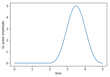
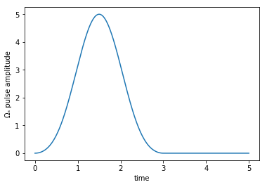
plot_pulse(H[1][1], tlist, 'Ωₚ')
plot_pulse(H[3][1], tlist, 'Ωₛ')
The imaginary parts are zero:
[11]:
assert np.all([H[2][1](t, None) == 0 for t in tlist])
assert np.all([H[4][1](t, None) == 0 for t in tlist])
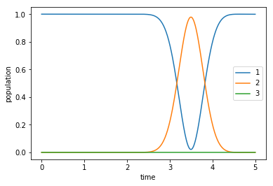
After assuring ourselves that our guess pulses appear as expected, we propagate the system using our guess. Since the pulses are temporally disjoint, we expect the first pulse to have no effect, whilst the second merely transfers population out of \(\Ket{1}\) into \(\Ket{2}\) and back again.
[12]:
guess_dynamics = objective.mesolve(tlist, e_ops=[proj1,proj2,proj3])
[13]:
def plot_population(result):
    fig, ax = plt.subplots()
    ax.plot(result.times, result.expect[0], label='1')
    ax.plot(result.times, result.expect[1], label='2')
    ax.plot(result.times, result.expect[2], label='3')
    ax.legend()
    ax.set_xlabel('time')
    ax.set_ylabel('population')
    plt.show(fig)
[14]:
plot_population(guess_dynamics)
Optimize
We now supply Krotov with all the information it needs to optimize, consisting of the objectives (maximize population in \(\Ket{3}\) at \(t_{1}\)), pulse_options (the initial shapes of our pulses and how they may be changed) as well as the propagator to use, optimization functional (chi_constructor), info_hook (processing occuring inbetween iterations of optimization) and the maximum number of iterations to perform, iter_stop. We will stop the optimization when
the error goes below \(10^{-3}\) or the fidelity has converged to within 5 digits.
[15]:
oct_result = krotov.optimize_pulses(
    [objective],
    pulse_options,
    tlist,
    propagator=krotov.propagators.expm,
    chi_constructor=krotov.functionals.chis_re,
    info_hook=krotov.info_hooks.print_table(
        J_T=krotov.functionals.J_T_re,
        show_g_a_int_per_pulse=True,
        unicode=False,
    ),
    check_convergence=krotov.convergence.Or(
        krotov.convergence.value_below(1e-3, name='J_T'),
        krotov.convergence.delta_below(1e-5),
        krotov.convergence.check_monotonic_error,
    ),
    iter_stop=15,
)
  iter.        J_T   g_a_int_1   g_a_int_2   g_a_int_3   g_a_int_4     g_a_int          J  Delta_J_T    Delta J  secs
      0   1.01e+00    0.00e+00    0.00e+00    0.00e+00    0.00e+00    0.00e+00   1.01e+00        n/a        n/a     1
      1   9.21e-01    1.09e-02    3.62e-05    1.08e-02    3.96e-05    2.18e-02   9.43e-01  -8.71e-02  -6.53e-02     2
      2   8.35e-01    1.08e-02    3.98e-05    1.07e-02    4.33e-05    2.15e-02   8.57e-01  -8.60e-02  -6.45e-02     2
      3   7.52e-01    1.05e-02    4.34e-05    1.03e-02    4.68e-05    2.09e-02   7.73e-01  -8.36e-02  -6.27e-02     2
      4   6.72e-01    1.01e-02    4.69e-05    9.84e-03    5.00e-05    2.00e-02   6.92e-01  -8.01e-02  -6.01e-02     2
      5   5.96e-01    9.54e-03    4.98e-05    9.26e-03    5.27e-05    1.89e-02   6.15e-01  -7.56e-02  -5.67e-02     2
      6   5.25e-01    8.91e-03    5.21e-05    8.60e-03    5.46e-05    1.76e-02   5.43e-01  -7.05e-02  -5.29e-02     2
      7   4.61e-01    8.22e-03    5.36e-05    7.89e-03    5.57e-05    1.62e-02   4.77e-01  -6.49e-02  -4.87e-02     2
      8   4.02e-01    7.49e-03    5.41e-05    7.16e-03    5.60e-05    1.48e-02   4.16e-01  -5.91e-02  -4.43e-02     2
      9   3.48e-01    6.76e-03    5.38e-05    6.43e-03    5.53e-05    1.33e-02   3.62e-01  -5.32e-02  -3.99e-02     2
     10   3.01e-01    6.04e-03    5.26e-05    5.72e-03    5.39e-05    1.19e-02   3.13e-01  -4.75e-02  -3.56e-02     2
     11   2.59e-01    5.34e-03    5.07e-05    5.05e-03    5.18e-05    1.05e-02   2.69e-01  -4.20e-02  -3.15e-02     2
     12   2.22e-01    4.70e-03    4.82e-05    4.42e-03    4.93e-05    9.22e-03   2.31e-01  -3.69e-02  -2.77e-02     2
     13   1.90e-01    4.10e-03    4.53e-05    3.85e-03    4.63e-05    8.04e-03   1.98e-01  -3.22e-02  -2.41e-02     2
     14   1.62e-01    3.56e-03    4.22e-05    3.34e-03    4.31e-05    6.98e-03   1.69e-01  -2.79e-02  -2.09e-02     2
     15   1.38e-01    3.07e-03    3.89e-05    2.88e-03    3.98e-05    6.03e-03   1.44e-01  -2.41e-02  -1.81e-02     2
[16]:
oct_result
[16]:
Krotov Optimization Result
--------------------------
- Started at 2019-03-01 01:46:52
- Number of objectives: 1
- Number of iterations: 15
- Reason for termination: Reached 15 iterations
- Ended at 2019-03-01 01:47:27
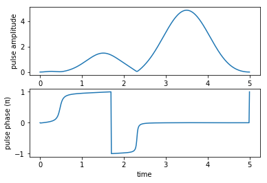
We appear to have found pulse-shapes that fulfill our objective, but what do they look like?
[17]:
def plot_pulse_amplitude_and_phase(pulse_real, pulse_imaginary,tlist):
ax1 = plt.subplot(211)
ax2 = plt.subplot(212)
amplitudes = [np.sqrt(x*x + y*y) for x,y in zip(pulse_real,pulse_imaginary)]
phases = [np.arctan2(y,x)/np.pi for x,y in zip(pulse_real,pulse_imaginary)]
ax1.plot(tlist,amplitudes)
ax1.set_xlabel('time')
ax1.set_ylabel('pulse amplitude')
ax2.plot(tlist,phases)
ax2.set_xlabel('time')
ax2.set_ylabel('pulse phase (π)')
plt.show()
print("pump pulse amplitude and phase:")
plot_pulse_amplitude_and_phase(
oct_result.optimized_controls[0], oct_result.optimized_controls[1], tlist)
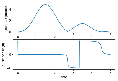
print("Stokes pulse amplitude and phase:")
plot_pulse_amplitude_and_phase(
oct_result.optimized_controls[2], oct_result.optimized_controls[3], tlist)
pump pulse amplitude and phase:
Stokes pulse amplitude and phase:
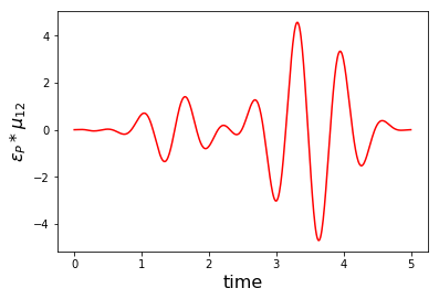
Once we have the optimized real and imaginary parts of the \(\Omega_P (t)\) and \(\Omega_P (t)\) functions we can retrieve the physical pulses \(\varepsilon _P (t)\) and \(\varepsilon _S (t)\) using their very definition.
[18]:
def plot_physical_field(pulse_re, pulse_im, tlist, case=None):
if case == 'pump':
w = 9.5
elif case == 'stokes':
w = 4.5
else:
print('Error: selected case is not a valid option')
return
ax = plt.subplot(111)
ax.plot(tlist,pulse_re*np.cos(w*tlist)-pulse_im*np.sin(w*tlist), 'r')
ax.set_xlabel('time', fontsize = 16)
if case == 'pump':
ax.set_ylabel(r'$\varepsilon_{P} * \mu_{12}$', fontsize = 16)
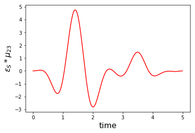
elif case == 'stokes':
ax.set_ylabel(r'$\varepsilon_{S} * \mu_{23}$', fontsize = 16)
plt.show()
print('Physical electric pump pulse in the lab frame:')
plot_physical_field(
oct_result.optimized_controls[0], oct_result.optimized_controls[1], tlist, case = 'pump')
print('Physical electric Stokes pulse in the lab frame:')
plot_physical_field(
oct_result.optimized_controls[2], oct_result.optimized_controls[3], tlist, case = 'stokes')
Physical electric pump pulse in the lab frame:
Physical electric Stokes pulse in the lab frame:
And how does the population end up in \(\Ket{3}\)?
[19]:
opt_dynamics = oct_result.optimized_objectives[0].mesolve(
    tlist, e_ops=[proj1, proj2, proj3])
[20]:
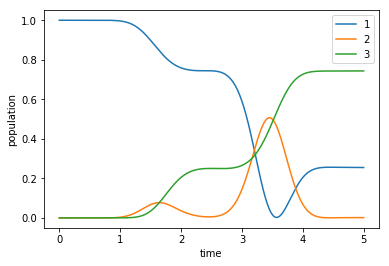
plot_population(opt_dynamics)